Directed search
This is the third turial in a series showcasing the functionality of the Exploratory Modeling workbench. Exploratory modeling entails investigating the way in which uncertainty and/or policy levers map to outcomes. To investigate these mappings, we can either use sampling based strategies (open exploration) or optimization based strategies (directed search).
In this tutorial, I will demonstrate in more detail how to use the workbench for directed search. We are using the same example as in the previous tutorials. When using optimization, it is critical that you specify for each Scalar Outcome the direction in which it should move. There are three possibilities: info which is ignored, maximize, and minimize. If the kind keyword argument is not specified, it defaults to info.
[1]:
from ema_workbench import RealParameter, ScalarOutcome, Constant, Model
from dps_lake_model import lake_model

model = Model("lakeproblem", function=lake_model)

# specify uncertainties
model.uncertainties = [
    RealParameter("b", 0.1, 0.45),
    RealParameter("q", 2.0, 4.5),
    RealParameter("mean", 0.01, 0.05),
    RealParameter("stdev", 0.001, 0.005),
    RealParameter("delta", 0.93, 0.99),
]

# set levers
model.levers = [
    RealParameter("c1", -2, 2),
    RealParameter("c2", -2, 2),
    RealParameter("r1", 0, 2),
    RealParameter("r2", 0, 2),
    RealParameter("w1", 0, 1),
]

# specify outcomes
model.outcomes = [
    ScalarOutcome("max_P", ScalarOutcome.MINIMIZE),
    ScalarOutcome("utility", ScalarOutcome.MAXIMIZE),
    ScalarOutcome("inertia", ScalarOutcome.MAXIMIZE),
    ScalarOutcome("reliability", ScalarOutcome.MAXIMIZE),
]

# override some of the defaults of the model
model.constants = [
    Constant("alpha", 0.41),
    Constant("nsamples", 150),
    Constant("myears", 100),
]
Using directed search with the ema_workbench requires platypus-opt. Please check the installation suggestions provided in the readme of the github repository. I personally either install from github directly
pip git+https://github.com/Project-Platypus/Platypus.git
or through pip
pip install platypus-opt
One note of caution: don’t install platypus, but platypus-opt. There exists a python package on pip called platypus, but that is quite a different kind of library.
There are three ways in which we can use optimization in the workbench: 1. Search over the decision levers, conditional on a reference scenario 2. Search over the uncertain factors, conditional on a reference policy 3. Search over the decision levers given a set of scenarios
Search over levers
Directed search is most often used to search over the decision levers in order to find good candidate strategies. This is for example the first step in the Many Objective Robust Decision Making process. This is straightforward to do with the workbench using the optimize method.
Note that I have kept the number of functional evaluations (nfe) very low. In real applications this should be substantially higher and be based on convergence considerations which are demonstrated below.
[2]:
from ema_workbench import MultiprocessingEvaluator, ema_logging

ema_logging.log_to_stderr(ema_logging.INFO)

with MultiprocessingEvaluator(model) as evaluator:
    results = evaluator.optimize(nfe=250, searchover="levers", epsilons=[0.1] * len(model.outcomes))
[MainProcess/INFO] pool started with 10 workers
298it [00:03, 75.48it/s]
[MainProcess/INFO] optimization completed, found 5 solutions
[MainProcess/INFO] terminating pool
The results from optimize is a DataFrame with the decision variables and outcomes of interest. This dataframe contains both the decision variables (c1-w1) and the outcomes (max_P-reliability). Each row is thus a single unique solution.
Note also that there might be a difference between the specified number of nfe (250 in this case) and the actual number of nfe. The default algorithm is population based and the nfe-based stopping condition is only checked after evaluating an entire generation.
[3]:
results
[3]:
| c1 | c2 | r1 | r2 | w1 | max_P | utility | inertia | reliability | |
|---|---|---|---|---|---|---|---|---|---|
| 0 | -0.682559 | 0.026569 | 1.738125 | 1.035683 | 0.514804 | 2.283760 | 1.655153 | 0.99 | 0.100133 |
| 1 | -1.667796 | -0.624652 | 0.914360 | 0.582130 | 0.243352 | 2.283627 | 1.778130 | 0.99 | 0.070000 |
| 2 | 1.869933 | 1.822573 | 0.798277 | 0.886831 | 0.686324 | 1.961235 | 0.615122 | 0.99 | 0.070000 |
| 3 | 0.442190 | 1.680330 | 0.989541 | 1.958483 | 0.979940 | 0.190612 | 0.523998 | 0.99 | 1.000000 |
| 4 | 0.096997 | 0.329009 | 0.500270 | 0.946994 | 0.344109 | 0.092322 | 0.233183 | 0.99 | 1.000000 |
Specifying constraints
It is possible to specify a constrained optimization problem. A model can have one or more constraints. A constraint can be applied to the model input parameters (both uncertainties and levers), and/or outcomes. A constraint is essentially a function that should return the distance from the feasibility threshold. The distance should be 0 if the constraint is met.
In the example below, we add a constrait saying that the value of the outcome max_P should be below 1. Given that this is a very simple constrain, I chose to use a lambda function to implement it. For more complicated constraints, you can also define your own function and pass that instead.
[4]:
from ema_workbench import Constraint

constraints = [Constraint("max pollution", outcome_names="max_P", function=lambda x: max(0, x - 1))]
[5]:
from ema_workbench import MultiprocessingEvaluator
from ema_workbench import ema_logging

ema_logging.log_to_stderr(ema_logging.INFO)

with MultiprocessingEvaluator(model) as evaluator:
    results = evaluator.optimize(
        nfe=250, searchover="levers", epsilons=[0.1] * len(model.outcomes), constraints=constraints
    )
[MainProcess/INFO] pool started with 10 workers
298it [00:03, 76.22it/s]
[MainProcess/INFO] optimization completed, found 2 solutions
[MainProcess/INFO] terminating pool
[6]:
results
[6]:
| c1 | c2 | r1 | r2 | w1 | max_P | utility | inertia | reliability | |
|---|---|---|---|---|---|---|---|---|---|
| 0 | 0.517330 | 0.130095 | 1.648766 | 1.005694 | 0.616171 | 0.093374 | 0.232173 | 0.99 | 1.0 |
| 1 | 0.034839 | 0.763078 | 1.654288 | 1.185964 | 0.783527 | 0.190797 | 0.510802 | 0.99 | 1.0 |
The new results with this simple constraint contains only a few solutions. This suggests that it is difficult to find solutions that are able to meet this constraint.
Seed analysis
Genetic algorithms rely on randomness in the search process. This implies that a single run of the algorithm does not tell you that much because the results might be due to randomness. It is thus best practice to allways repeat the optimization for several different seeds and next merge the results across the different optimizations. This is supported by the workbench. We first need to run multiple optimization like this:
[7]:
results = []
with MultiprocessingEvaluator(model) as evaluator:
    # we run 5 seperate optimizations
    for _ in range(5):
        result = evaluator.optimize(
            nfe=5000, searchover="levers", epsilons=[0.05] * len(model.outcomes)
        )
        results.append(result)
[MainProcess/INFO] pool started with 10 workers
5036it [00:37, 133.58it/s]
[MainProcess/INFO] optimization completed, found 25 solutions
5058it [00:36, 140.03it/s]
[MainProcess/INFO] optimization completed, found 41 solutions
5049it [00:35, 140.43it/s]
[MainProcess/INFO] optimization completed, found 26 solutions
5054it [00:35, 140.87it/s]
[MainProcess/INFO] optimization completed, found 16 solutions
5052it [00:36, 140.17it/s]
[MainProcess/INFO] optimization completed, found 30 solutions
[MainProcess/INFO] terminating pool
We now have the results for each of the five different runs of the optimization. The next step is to combine these into a singe comprehensive set. Since by default the workbench uses ε-NSGAII, it makes sense to also merge the results across the seeds using an ε-nondominated sort.
[11]:
from ema_workbench.em_framework.optimization import epsilon_nondominated, to_problem

problem = to_problem(model, searchover="levers")
epsilons = [0.05] * len(model.outcomes)
merged_archives = epsilon_nondominated(results, epsilons, problem)
[9]:
merged_archives.shape
[9]:
(34, 9)
As can be seen, the new merged archive contains 34 solutions. Which is is quite a bit smaller than the sum of solutions across the 5 seeds. This implies that many of the solutions found in each seed land in the same ε-gridcell.
Tracking convergence
An important part of using many-objective evolutionary algorithms is to carefully monitor whether they have converged to the best possible solutions. Various different metrics can be used for this. Some of these metrics must be collected at runtime, such as ε-progress. Others, like hypervolume, are better calculated after the optimization has been completed. The metrics that are better calculated after the optimization require, however, storing the state of the archive over the course of the optimization. Both types of metrics are supported by the workbench.
[23]:
from ema_workbench.em_framework.optimization import ArchiveLogger, EpsilonProgress

# we need to store our results for each seed
results = []
convergences = []

with MultiprocessingEvaluator(model) as evaluator:
    # we run again for 5 seeds
    for i in range(5):
        # we create 2 covergence tracker metrics
        # the archive logger writes the archive to disk for every x nfe
        # the epsilon progress tracks during runtime
        convergence_metrics = [
            ArchiveLogger(
                "./archives",
                [l.name for l in model.levers],
                [o.name for o in model.outcomes],
                base_filename=f"{i}.tar.gz",
            ),
            EpsilonProgress(),
        ]

        result, convergence = evaluator.optimize(
            nfe=50000,
            searchover="levers",
            epsilons=[0.05] * len(model.outcomes),
            convergence=convergence_metrics,
        )

        results.append(result)
        convergences.append(convergence)
[MainProcess/INFO] pool started with 10 workers
50061it [06:17, 132.46it/s]
[MainProcess/INFO] optimization completed, found 39 solutions
50117it [06:23, 130.56it/s]
[MainProcess/INFO] optimization completed, found 31 solutions
50081it [06:11, 134.92it/s]
[MainProcess/INFO] optimization completed, found 32 solutions
50085it [05:57, 139.98it/s]
[MainProcess/INFO] optimization completed, found 37 solutions
50062it [1:12:08, 11.57it/s]
[MainProcess/INFO] optimization completed, found 33 solutions
[MainProcess/INFO] terminating pool
Varous metrics are provied by platypus. For details on these metrics see e.g., Zatarain-Salazar et al (2016) and Gupta et al (2020) for hypervolume, generational distance and additive \(\epsilon\)-indicator; Hadka and Reed (2012) for spacing; and Hadka and Reed (2013) for \(\epsilon\)-pgrogress. To use these metrics, we first need to load the archives into memory. Next, these metrics need a set of platypus solutions, instead of the dataframes that the workbench has stored. Moreover, most of these metrics need a reference set. The reference set, typically, is the union of best solutions found across the seeds and next filtered using an ε-nondominated sort. All these steps are supported by the workbench as shown below.
[24]:
all_archives = []

for i in range(5):
    archives = ArchiveLogger.load_archives(f"./archives/{i}.tar.gz")
    all_archives.append(archives)
[25]:
from ema_workbench import (
    HypervolumeMetric,
    GenerationalDistanceMetric,
    EpsilonIndicatorMetric,
    InvertedGenerationalDistanceMetric,
    SpacingMetric,
)
from ema_workbench.em_framework.optimization import to_problem

problem = to_problem(model, searchover="levers")

reference_set = epsilon_nondominated(results, [0.05] * len(model.outcomes), problem)

hv = HypervolumeMetric(reference_set, problem)
gd = GenerationalDistanceMetric(reference_set, problem, d=1)
ei = EpsilonIndicatorMetric(reference_set, problem)
ig = InvertedGenerationalDistanceMetric(reference_set, problem, d=1)
sm = SpacingMetric(problem)


metrics_by_seed = []
for archives in all_archives:
    metrics = []
    for nfe, archive in archives.items():
        scores = {
            "generational_distance": gd.calculate(archive),
            "hypervolume": hv.calculate(archive),
            "epsilon_indicator": ei.calculate(archive),
            "inverted_gd": ig.calculate(archive),
            "spacing": sm.calculate(archive),
            "nfe": int(nfe),
        }
        metrics.append(scores)
    metrics = pd.DataFrame.from_dict(metrics)

    # sort metrics by number of function evaluations
    metrics.sort_values(by="nfe", inplace=True)
    metrics_by_seed.append(metrics)
Now that we have calculated all our metrics, we can visualize them using matplotlib.
[26]:
sns.set_style("white")
fig, axes = plt.subplots(nrows=6, figsize=(8, 12), sharex=True)

ax1, ax2, ax3, ax4, ax5, ax6 = axes

for metrics, convergence in zip(metrics_by_seed, convergences):
    ax1.plot(metrics.nfe, metrics.hypervolume)
    ax1.set_ylabel("hypervolume")

    ax2.plot(convergence.nfe, convergence.epsilon_progress)
    ax2.set_ylabel("$\epsilon$ progress")

    ax3.plot(metrics.nfe, metrics.generational_distance)
    ax3.set_ylabel("generational distance")

    ax4.plot(metrics.nfe, metrics.epsilon_indicator)
    ax4.set_ylabel("epsilon indicator")

    ax5.plot(metrics.nfe, metrics.inverted_gd)
    ax5.set_ylabel("inverted generational\ndistance")

    ax6.plot(metrics.nfe, metrics.spacing)
    ax6.set_ylabel("spacing")

ax6.set_xlabel("nfe")


sns.despine(fig)

plt.show()
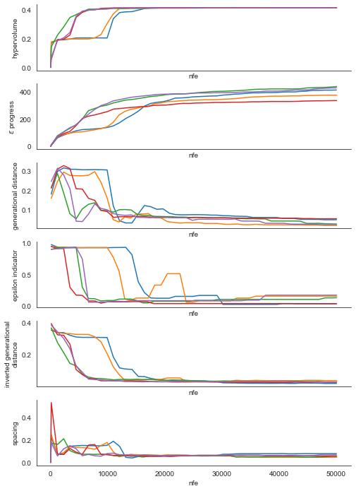
As we can see, for this problem across all the metrics and for each of the seeds we see that the line stabilizes which is indicative of convergence. The fact that the lines for each of the seeds stabilizes at roughly the same value moreover suggests that the seeds are converging to similar sets of solutions.
Changing the reference scenario
The workbench offers control over the reference scenario or policy under which you are performing the optimization. This makes it easy to apply multi-scenario MORDM (Watson & Kasprzyk, 2017;Eker & Kwakkel, 2018;Bartholomew & Kwakkel, 2020). Alternatively, you can also use it to change the policy for which you are applying worst case scenario discovery (see below).
reference = Scenario('reference', b=0.4, q=2, mean=0.02, stdev=0.01)

with MultiprocessingEvaluator(lake_model) as evaluator:
    results = evaluator.optimize(searchover='levers', nfe=1000,
                       epsilons=[0.1, ]*len(lake_model.outcomes),
                       reference=reference)
Search over uncertainties: worst case discovery
Up till now, the focus has been on applying search to find promising candidate strategies. That is, we search through the lever space. However, there might also be good reasons to search through the uncertainty space. For example to search for worst case scenarios (Halim et al, 2015). This is easily achieved as shown below. We change the kind attribute on each outcome so that we search for the worst outcome and specify that we would like to search over the uncertainties instead of the levers.
Any of the foregoing additions such as constraints or convergence works as shown above. Note that if you would like to to change the reference policy, reference should be a Policy object rather than a Scenario object.
[7]:
# change outcomes so direction is undesirable
minimize = ScalarOutcome.MINIMIZE
maximize = ScalarOutcome.MAXIMIZE

for outcome in model.outcomes:
    if outcome.kind == minimize:
        outcome.kind = maximize
    else:
        outcome.kind = minimize

with MultiprocessingEvaluator(model) as evaluator:
    results = evaluator.optimize(
        nfe=1000, searchover="uncertainties", epsilons=[0.1] * len(model.outcomes)
    )
[MainProcess/INFO] pool started with 10 workers
1090it [00:09, 116.02it/s]
[MainProcess/INFO] optimization completed, found 8 solutions
[MainProcess/INFO] terminating pool
Parallel coordinate plots
The workbench comes with support for making parallel axis plots through the parcoords module. This module offers a parallel axes object on which we can plot data.
The typical workflow is to first instantiate this parallel axes object given a pandas dataframe with the upper and lower limits for each axes. Next, one or more datasets can be plotted on this axes. Any dataframe passed to the plot method will be normalized using the limits passed first. We can also invert any of the axes to ensure that the desirable direction is the same for all axes.
[9]:
from ema_workbench.analysis import parcoords

data = results.loc[:, [o.name for o in model.outcomes]]

# get the minimum and maximum values as present in the dataframe
limits = parcoords.get_limits(data)

# we know that the lowest possible value for all objectives is 0
limits.loc[0, ["utility", "inertia", "reliability", "max_P"]] = 0
# inertia and reliability are defined on unit interval, so their theoretical maximum is 1
limits.loc[1, ["inertia", "reliability"]] = 1

paraxes = parcoords.ParallelAxes(limits)
paraxes.plot(data)
paraxes.invert_axis("max_P")
plt.show()
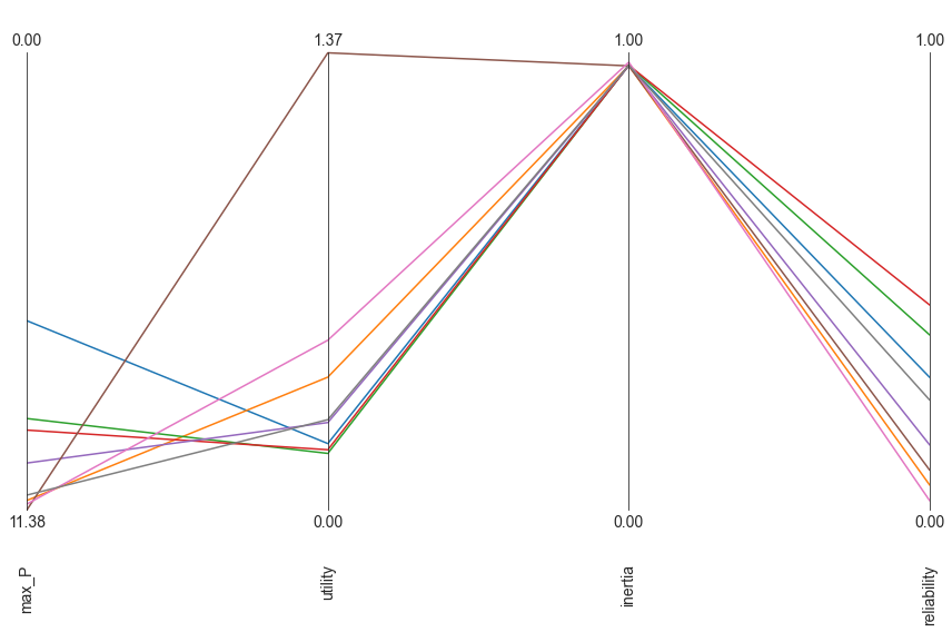
The above parallel coordinate plot shows the results from the worst case discovery. The worst possible solution would be a straight line at the bottom. A key insight from this result is that there seems to be a trade-off between max_P and utility. This can be inferred from the crossing lines between these two axes.
Robust Search
In the foregoing, we have been using optimization over levers or uncertainties, while assuming a reference scenario or policy. However, we can also formulate a robust many objective optimization problem (Kwakkel et al. 2015; Bartholomew et al. 2020), where we are going to search over the levers for solutions that have robust performance over a set of scenarios. To do this with the workbench, there are several steps that one has to take.
First, we need to specify our robustness metrics. A robustness metric takes as input the performance of a candidate policy over a set of scenarios and returns a single robustness score. For a more in depth overview, see McPhail et al. (2018). In case of the workbench, we can use the ScalarOutcome class for this. We need to specify the name of the robustness metric a function that takes as input a numpy array and returns a single number, and the model outcome to which this function should be applied.
Below, we use a percentile based robustness metric, which we apply to each model outcome.
[20]:
import functools

# our robustness functions
percentile10 = functools.partial(np.percentile, q=10)
percentile90 = functools.partial(np.percentile, q=90)

# convenient short hands
MAXIMIZE = ScalarOutcome.MAXIMIZE
MINIMIZE = ScalarOutcome.MINIMIZE

robustnes_functions = [
    ScalarOutcome(
        "90th percentile max_p", kind=MINIMIZE, variable_name="max_P", function=percentile90
    ),
    ScalarOutcome(
        "10th percentile reliability",
        kind=MAXIMIZE,
        variable_name="reliability",
        function=percentile10,
    ),
    ScalarOutcome(
        "10th percentile inertia", kind=MAXIMIZE, variable_name="inertia", function=percentile10
    ),
    ScalarOutcome(
        "10th percentile utility", kind=MAXIMIZE, variable_name="utility", function=percentile10
    ),
]
Next, we have to generate the scenarios we want to use. Below we generate 10 scenarios, which we will keep fixed over the optimization. The exact number of scenarios to use is to be established through trial and error. Typically it involves balancing computational costs of more scenarios, with the stability of the robustness metric over the number of scenarios
[23]:
from ema_workbench.em_framework import sample_uncertainties

n_scenarios = 10
scenarios = sample_uncertainties(model, n_scenarios)
With the robustness metrics specified, and the scenarios, sampled, we can now perform robust many-objective optimization. Below is the code that one would run. Note that this is computationally very expensive since each candidate solution is going to be run for ten scenarios before we can calculate the robustness for each outcome of interest.
[24]:
from ema_workbench.em_framework import ArchiveLogger

nfe = int(5e4)
with MultiprocessingEvaluator(model) as evaluator:
    robust_results = evaluator.robust_optimize(
        robustnes_functions,
        scenarios,
        nfe=nfe,
        epsilons=[
            0.025,
        ]
        * len(robustnes_functions),
    )
[MainProcess/INFO] pool started with 10 workers
50039it [2:10:57,  6.37it/s]
[MainProcess/INFO] optimization completed, found 29 solutions
[MainProcess/INFO] terminating pool
We can now again visualize the results using a parallel coordinate plot. Note that we are visualizing the robustness scores rather than the outcomes of interest as specified in the underlying model.
[29]:
from ema_workbench.analysis import parcoords


data = robust_results.loc[:, [o.name for o in robustnes_functions]]
limits = parcoords.get_limits(data)

paraxes = parcoords.ParallelAxes(limits)
paraxes.plot(data)
paraxes.invert_axis("90th percentile max_p")
plt.show()
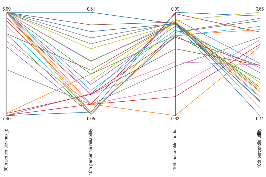
What we can see in this parallel axis plot is that there is a clear tradeoff between robust high reliability and robsut low maximum polution. Likewise with inertia and utility. This can be seen from the crossing lines between these respective axes.
[ ]: